The Mono Lake Case study
Submit the lab before Sunday May 31st 2026, 20:00
Introduction
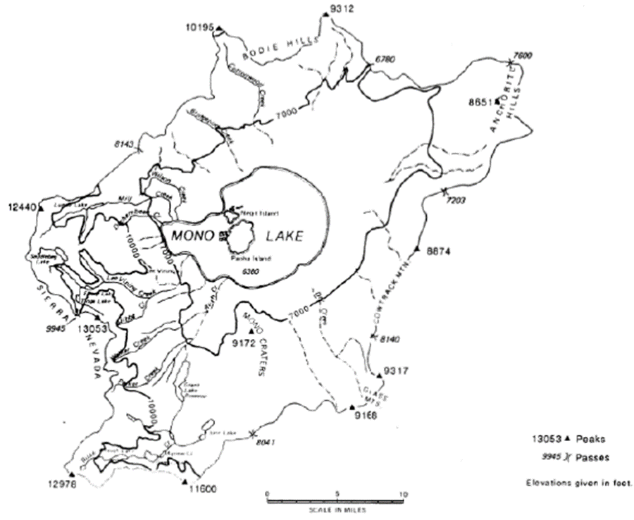
Mono Lake is an ancient saline lake situated in eastern California, near the Sierra Nevada. Due to its lack of a natural outlet, the lake loses water solely through evaporation, making it highly susceptible to fluctuations in water inflow. In 1941, the Los Angeles Department of Water and Power commenced diverting water from the lake’s tributary streams to cater to the expanding city. Over subsequent decades, these diversions led to a significant reduction in the lake level (over 40 feet by the 1980s).
This decline had severe ecological repercussions. As the lake’s size diminished, its salinity increased, endangering the brine shrimp that are fundamental to the food web. Migratory birds that depend on the lake for nesting and feeding faced substantial risks. The exposure of lake beds created land bridges to islands where birds nest, allowing predators such as coyotes to access and disrupt breeding colonies. Furthermore, the dried lake bed became a source of windblown dust, contributing to air quality issues.
Public concern and legal interventions eventually resulted in revised policies. In 1994, the California State Water Board mandated that a portion of the water must remain in the lake’s tributaries, establishing a target to elevate Mono Lake to a more sustainable level. The public initative that ultimately led to the legislative changes is still active and is actively monitoring lake levels closely: https://www.monolake.org/.
In this lab, you will employ Vensim to examine the feedback loops and time delays characteristic of the Mono Lake crisis. By constructing and simulating a simplified model of the lake system, you will develop an understanding of the interaction between human activity and natural systems, and the impact of policy decisions on long-term outcomes.
General structure and submission
The lab is subdivided into several parts, which we will address on different days. Along the way we will ask you to make some smaller calculations, export some graphics from Vensim and answer some questions. Please compile all answers in a document, which you later upload in moodle in form of a pdf. You are encouraged to work together with your fellow lab mates (e.g., in groups of 2-3) to implement the model and compare your calculations, but you need to submit your own version of the lab report.
Exercise I: Implementation of the Mono Lake system model in Vensim
In Figure 2 you find a stock-and-flow diagram of the Mono Lake hydrological model. In this first task, we ask you to implement this model in Vensim using the knowledge you gained in last week’s exercise. For the implementation, remember that the symbology in Vensim is slightly different from the one used below. Specifically, in the below example circles  represent auxiliary variables which in Vensim are incorporated using the button
  . The
. The  symbol below are flows, built in Vensim as
  . Stocks and links below have the same notation in Vensim
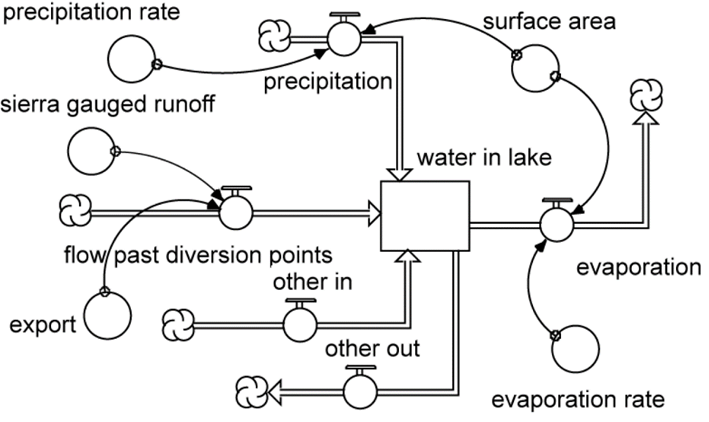
After you implement the model in Vensim, you need to parameterize all stocks and flows. Do this using the parameters provided in Table 1, i.e., by filling the initial values and equations if needed. The units in Vensim (i.e., in the variable information that appears once you click on an object with the equation tool  ) are only for visual purposes and will only appear on graphs – this means, that before running any simulation you will need to check whether the units between stocks and flows are provided at the same scale. If they do differ in scale (e.g., hectare vs. acre) you will need to convert the units manually. In our example here, no conversion is necessary. Yet, the units provided there will give you an idea on how to set some of the equations.
| Parameter | Value | Unit of measurement |
|---|---|---|
| Surface Area | 39 | KA (1000 acres) |
| Reservoir volume | 2,228 | KAF (1000 acre-foot) |
| Gauged runoff from the Sierra Mountain range | 150 | \(KAF *yr^-1\) |
| Other inflows | 47.6 | \(KAF *yr^-1\) |
| Diversion of water (export) towards the Los Angeles agglomeration | 100 | \(KAF *yr^-1\) |
| Other outflows (accumulated total) | 33.6 | \(KAF *yr^-1\) |
| Precipitation rate | 0.67 | \(ft *yr^-1\) |
| Evaporation rate | 3.75 | \(ft *yr^-1\) |
Once you set up your model and provided all parameters, we want to you to run a simulation from 1990 to 2030 in time intervals of 1 year (Δt = 1). Go to the Model –> Settings and check whether Euler is selected as integration technique. In the same menu, under Time Bounds the box Save results every TIME STEP should be ticked (this is a technical detail concerning how the model file is stored – for the moment, we will neglect this detail). After the simulation, carefully examine the output and address the questions below for your written report.
Exercise II: Implementing relationships between variables inside the model
The first version of the model has clearly some issues. For example, currently the model is designed in a way that it assumes the lake were shaped like a cylinder as the water surface does not change with changing reservoir volume. More realistically would be to model the basin in form of a shallow cup, which means that the surface area of the lake decreases with decreasing water volume.
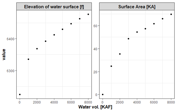
In this exercise we will address this issue and modify the model by implementing a response of the surface area (i.e., changes therein) to changes in the stock water volumes. In Vensim, one can do that through the integration of so-called lookup tables into the model. In a look-up table one can establish relationships between two (or more) variables, e.g., between water volume and surface area. You can find the required input for such a look-up table in Table 2 and the corresponding visualization in Figure 3.
| Water volume in reservoir [KAF] | Surface area [KA] | Elevation of water surface [ft a.s.l.] |
|---|---|---|
| 0 | 0 | 6224 |
| 1000 | 24.7 | 6335 |
| 2000 | 35.3 | 6369 |
| 3000 | 48.6 | 6392 |
| 4000 | 54.3 | 6412 |
| 5000 | 57.2 | 6430 |
| 6000 | 61.6 | 6447 |
| 7000 | 66.0 | 6463 |
| 8000 | 69.8 | 6477 |
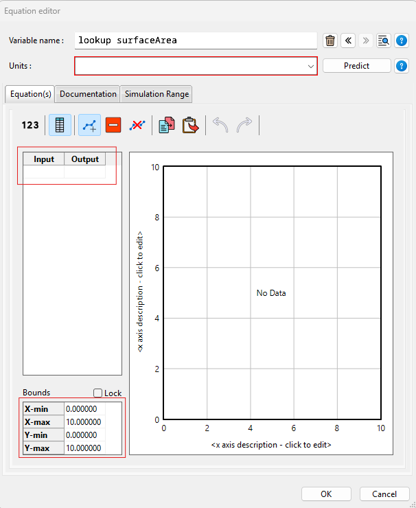
To implement such a lookup table in Vensim you will need to add a variable to the model that will be used as a lookup (here called: lookup_surfaceArea). Open the equations dialog for this variable (using the ) button) and change the type of the variable to LookUp (Figure 4).
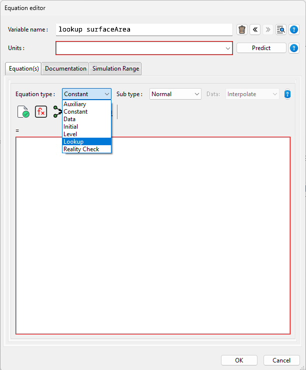
Now you need to establish the relationship between the variable surface area and water volume for this lookup. You do this, by navigating to the As Graph menu and by entering the values into the table that is shown. Make sure you assign the variable water volume as x (i.e., Input) and surface area as y (i.e., Output). Vensim will directly translate these values into the corresponding visualization using linear interpolation between the values (Figure 5). Click okay and you’ll see that the information that you just entered is encoded in the Equations text box. After that, close the ) dialog.
Now we need to make changes to the model structure in order to make use of the look-up that we just created. The variable SurfaceArea now contains values that correspond to the actual surface area of the lake depending on the actual water volume – all provided through the lookup-function that we built. Now, all is left is to add a link between the variable WaterVolume and the variable SurfaceArea:
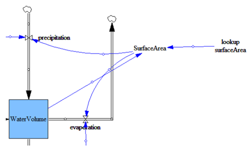
WaterVolume to SurfaceArea..
Next, change the equation of the variable SurfaceArea as indicated below. This function will pass the current water volume to the look-up variable which will return the corresponding surface area which then is used to determine evaporation and precipitation. Use a table or a graph module to visualize the changes in the surface area.
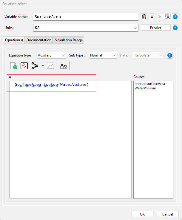
SurfaceArea.
Now, that we are all set, run the model for the period 1990-2090 using a time interval of 1 year applying Euler’s integration (like in exercise I).
Before we proceed to exercise 3, I want you to make one more modification to the model. Specifically, please implement now the water surface elevation (in ft. a.s.l.) into the model using a look-up table as before. This variable, which represents the elevation of the water surface is also function of the lake’s water level. Re-run the experiment and answer the question below.
Exercise III: Salinity and its impact on evaporation
Evaporation is not only dependent on the surface area of Mono Lake, but it additionally depends on the salinity and the density of the lake’s water. For example, highly saline water tends to evaporate more slowly – which means that the higher the salinity of the water is, the lower is the effective evaporation. The density of water, on the other hand, depends on the number of solids that are dissolved in water. The effect of increasing density can be expressed by applying the formula of specific gravity \(SG\):
\[ SG = \frac{V_{reservoir} * \rho_{freshwater} + m_{dissolved}}{V_{reservoir} * \rho_{freshwater}} \] where \(V_{reservoir}\) is the water volume (KAF), \(\rho_{freshwater}\) corresponds to the freshwater reference (density) fixed at 1.359 Mio. t per KAF, and where \(m_{dissolved}\) is the total amount of solids dissolved in the lake, which equals here to 230 Mio t. The relationship between specific gravity (without unit) and evaporation, expressed through the effective evaporation rate, is shown in Table 3.
| Specific gravity | Effective evaporation rate coefficient |
|---|---|
| 1.00 | 1.00 |
| 1.05 | 0.963 |
| 1.10 | 0.962 |
| 1.15 | 0.880 |
| 1.20 | 0.833 |
| 1.25 | 0.785 |
| 1.30 | 0.737 |
| 1.35 | 0.688 |
| 1.40 | 0.640 |
Your task now is to implement this additional detail to your model using the techniques you learned in the previous exercises. After that, re-run the simulation for the period 1990-2090. Once you have done this, please answer the questions below.
Exercise IV: Mono Lake policy questions
Now that we have a proper model, we want to explore a number of what-if scenarios. Consider a sea level elevation of 6340 ft asl to be set as a policy threshold level, below which no further water from the lake is allowed to be drained. Explore the following what-if scenarios considering this threshold:
Assume the default exports to be allowed until the threshold is exceeded. After that, no exports are allowed.
Assume an intervention scheme, where a maximum water export of
100 KAF/yris allowed if the elevation is above an upper threshold value (6390 ft. asl), water export is disallowed below a lower threshold level (6380 ft. asl), and export changes gradually between the maximum allowed value and zero in between these elevations
You will have to use a conditional statement in your export variable to implement this. The conditional statement in [Vensim].{smallcaps} looks like this: IF THEN ELSE(condition, value if condition TRUE, value if condition FALSE)