Introduction to Vensim
No formal submission needed, but please make sure that you know the techniques of this lab by heart
Introduction
Welcome to the first lab with Vensim. This assignment gives you the opportunity to get used to the modelling environment that we will use during large parts of the course. As such, several of the exercises will appear simple to you and you probably will finish them within a relatively short time. Below, we will guide you through each individual exercise using screenshots. At the end of each exercise, we will ask you to either extract some numbers from the output of Vensim or generate screenshots of one or more graphs. We will then discuss these in the classroom today. In the future, you will have to prepare written reports.
Preparation work
Please open Vensim either on the seminar server or on your local machine. Make yourself familiar with the environment. As a general rule you should for each individual model (i.e., from each exercise today and in future labs) create an individual folder to avoid overwriting results. For less complex models and simulations this may seem unnecessary, but we want to you adapt a working habit that is compatible with more complex modelling tasks in the future.
Some basic terminology and functions in Vensim
During the presentation, we talked about terminology, such as stocks, flows, etc. Below you find a table for the name of each term and the tool name in Vensim including the symbol.
| Lecture Term | Tool in Vensim | Icon to look for |
|---|---|---|
| Stocks | Stock tool |  |
| Auxiliary Variables | Variable tool |  |
| Flows | Flow tool |  |
| Connectors | Arrow tool |  |
Exercise I: A simple model
Navigate to Vensim and create a new model. You can already choose here the simulation period (we will use 2000-2050 in 1-yr intervals), but you leave this for now and edit it later.
 Once you have created the model, you will see a blank sketch. The first thing we want to do is to add a stock and a flow. To do this, click on the stock tool and place it in the sketch. You can double-click on the stock to edit its name. Name it
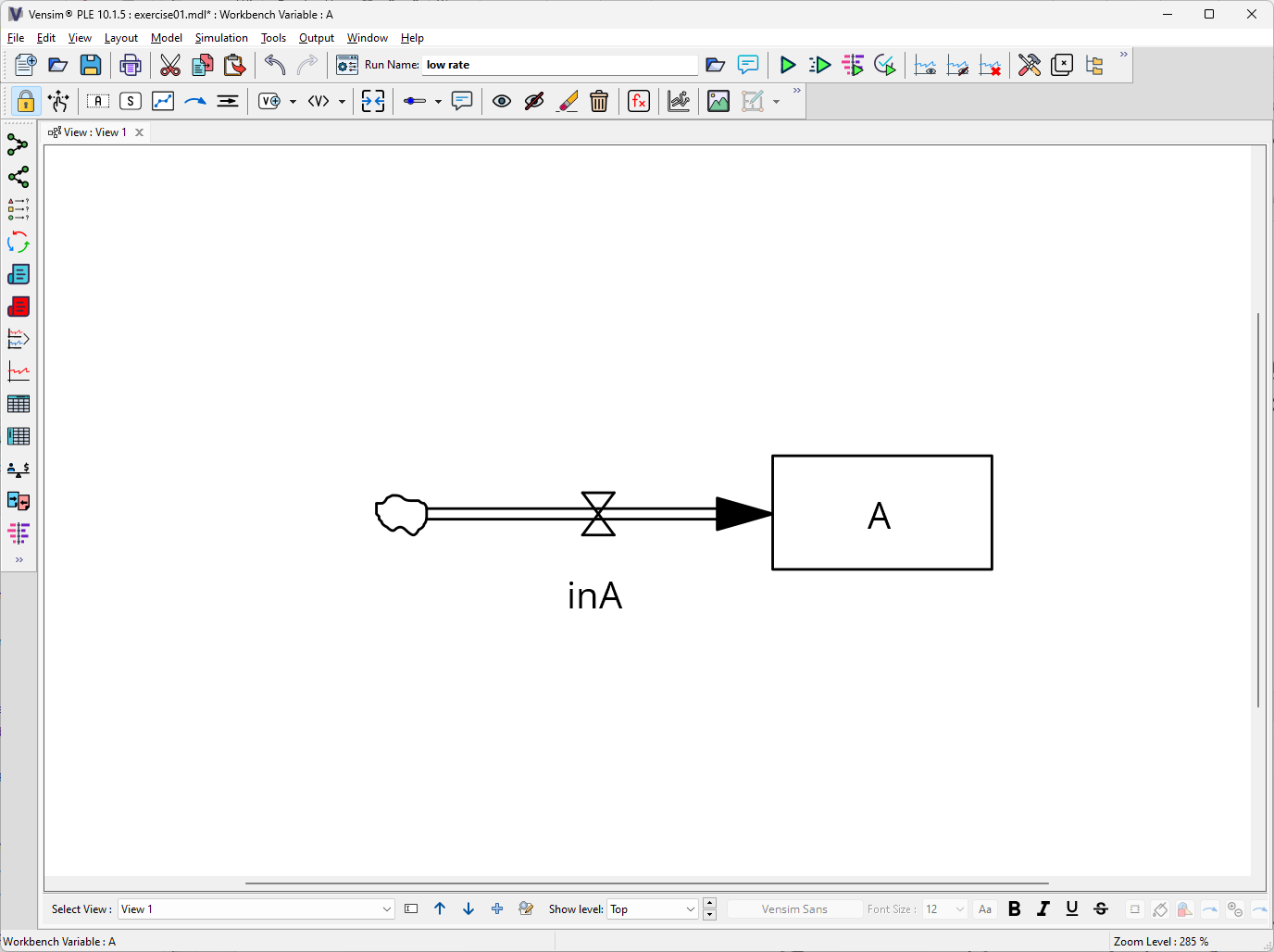
 A. Next, click on the flow tool and place it in the sketch. Connect the flow to the stock by clicking on the stock first and then on the flow. You can double-click on the flow to edit its name. Name it in_A. Your model should look like the example below:
Now, we need to set the variables. We do this using the equation tool  . In this window, we are now setting all the variables and boundary conditions for our model. To do this, click on the icon in the top menu. Now, you will see that the variables that we can edit in this model (i.e.,
 A and in_A). If you click on one of them, a dialogue box opens. In this example, I clicked on the variable in_A.
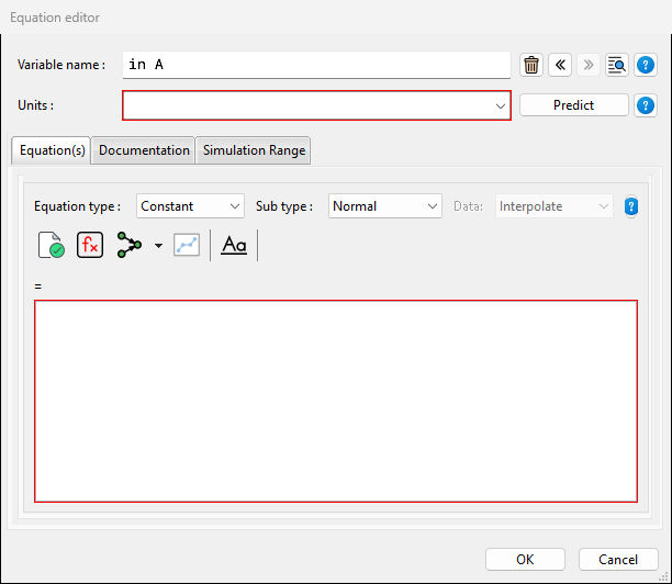
As a an important rule/orientation, you can note down, that for flows we have to define an equation, whereas for stocks we define an initial value, which represents the value this stock has at the beginning of the simulation period. Parameterize the model now as follows: in_A = 10 and A = 0. The initial value of the stock is set to zero, because we want to see how the stock develops over time.
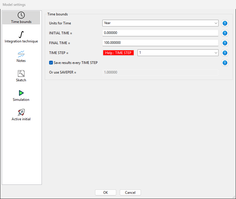
What is left is defining the boundary parameters. For this model, we need to edit INITIAL TIME, FINAL TIME and TIME STEP. If you have not done this at the beginning when creating the model, you can now go back to it via Model $\rightarrow$ Settings and edit INITIAL TIME = 2000, FINAL TIME = 2050, and TIME STEP = 1. Make sure that for all variables and boundary conditions the unit is set to Year. You should save now the model and run the simulation. To do so, hit the  button to run your first simulation in Vensim. If no error message pops up, then your model ran successfully. Let’s check our output. Click on the
  button (if not already activated) and click on
 A to activate it. Now check out the tools on the left  and
and  to see and visualize the simulation results. What model behavior do you observe?
Exercise II: Expand the model
In this exercise we want you to adapt the model from exercise I. To do this, make sure that you save the model in a new folder and with a new name to avoid overwriting the results. You can do this via File \(\rightarrow\) Save As. Once saved, adapt your model as follows: add a new stock B and an outflow out_B. Choose suitable parameters for the initial values of B and out_B. Simulate the model and examine the system behavior by visualizing a graph that shows stocks A and B. You can do this by holding the SHIFT-Button when selecting multiple stocks. Once you are done, answer the following question.
Exercise III: Introducing feedbacks
In this exercise we add complexity to simple flow models by adding auxiliary variables as well as causal links to the model. To do that, repeat what we did in exercise I and implement stock A and flow in_A in the same way (however: do not specify them yet!). Afterwards add an auxiliary variable valueA and a causal link (blue arrows) by clicking on the respective from and to element in the sketch (Hint: curved arrows are created by clicking on the from-element, then on an empty spot on the sketch, then on the to-element). Do this between A and inA and between valueA and in_A. Your model should look similar to the one below:
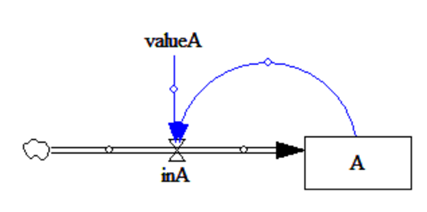
Now we focus on the specification. Set as initial values A = 10 to 10 and valueA = 0.1. For in_A we don’t specify a constant value, but instead we define it as in_A = valueA * A. Define the model settings (INITIAL_TIME, etc.) similar to exercise I. We could run the model now, but instead lets add some graphical IO element to our sketch and have a graph directly presented at the end of the model run. To do that, click first the Control Panel button ( and select the Graphs tab. Because there were no graphs yet defined, we have to click New. Give the graph a Name and a Title of your choice. Then select as values for the x-Axis the variable Time and on the bottom the variable A that we want to visualize. Click OK. The defined graph should now show up in the control panel. If so, everything done here, click „Close“.
Back in the sketch, select the menu that allows you to add graphs. You can find it in the top menu and it can have the  icon or the
  icon. Then, click in an empty location of your sketch; the Input Output Object settings dialog should appear. Here, select Output custom graph as Object Type and then the graph we defined in the previous step. Click OK. You’ll see that the blank graph is now added to the sketch. Place it into a location of your choice. After that, we are ready to run the simulation. The outputs are now directly visualized. Examine the graph and answer the question below.
In the next step we want to (a) modify the properties of valueA. Modify this variable by defining a minimum value of 0, a maximum value of 10, and the increment to 0.1. After confirming these changes, run the simulation again. This time, however, use the SyntheSim function  to do so. Observe the dynamic adjustment of the graph by moving the slider for
 valueA There is nothing to report for this part of the exercise, but I encourage you to play around with it for a little.
Exercise IV: A real-world application
In this fourth exercise we are moving away from purely abstract (and simple) simulation models towards a real-world application. Specifically, we will parameterize a population model for Papua New Guinea. Below you find the concept of a very basic population model with one stock (i.e., the variable we are interested in), two flows and two auxiliary variables.
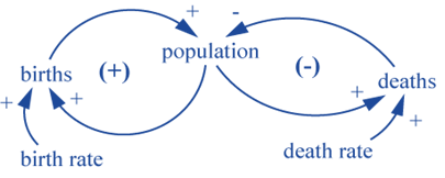
Your task is to build this model in Vensim using the parameterizations from the table below for the period 2010 to 2100. After that, answer the questions below the table. After that, please answer the two questions.
| Variable | Value |
|---|---|
| Population estimate in 2010 | 6,064,515 |
| Birth rate (per 1000 inh.) | 24.0 |
| Death rate (per 1000 inh.) | 6.5 |
Exercise V: Non-linear response modelling
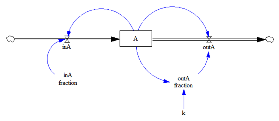
In our last exercise we will implement a non-linear response to our models. As a first step, implement the model scheme below in Vensim. As initial values for the various stocks and flows please consult the table below the model scheme.
| Variable | Value |
|---|---|
| A (initial value) | 1 |
| inA | A * inA fraction |
| outA | A * outA fraction |
| inA fraction | 0.25 (min: 0.001, max: 0.5) |
| outA fraction | A * k |
| k | 0.0025 (min: 0.001, max: 0.05) |
For the visualization I want you to create two I/O chart objects inside the sketch: one to visualize changes in the stock, and one to visualize the in/out rates (Hint: to add more than one variable in a graph, simply add more than one element inside the graph definition). Run the model using these model settings. Describe the sensitivity of the models to changes in k applying different values for k using the simulate button.